
What should roboticists care about when designing / controlling tendon-driven structures, like robot hands or arms? This post covers the fundamental concept behind such mechanisms- in particular, the tendon Jacobian. Harnessing this will make the difference between a well-behaving robot that can output sufficient torque throughout the joint range, or a bad design whose output torque suddenly diminishes at random postures. There is even an interactive demo where you can “design” a simple tendon-driven joint! I believe that what I cover here should be standard knowledge for anyone designing or controlling such tendon-driven structures.
This is a blog post version of the lecture notes that I created for teaching the Soft and Biohybrid Robotics course at ETH Zurich. The LaTeX source for the original lecture notes can be viewed here on Overleaf or on GitHub.
Setup and notation
Let
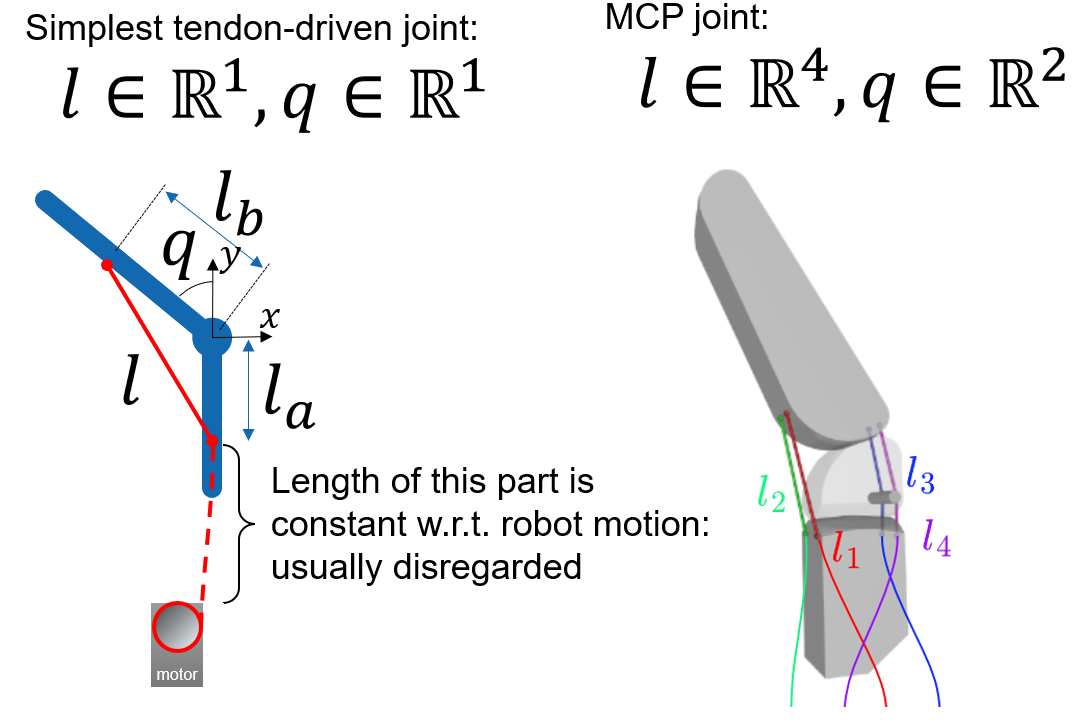
- \(\mathbf{q} \in \mathbb{R}^n\) be the vector of joint coordinates,
- \(\mathbf{l}\in \mathbb{R}^m\) be the vector of tendon lengths,
- \(\mathbf{f} \in \mathbb{R}^m\) be the vector of tendon tensions (\(f_i \ge 0\) because tendons can only pull),
- \(\mathbf{\tau} \in \mathbb{R}^n\) be the vector of generalized joint torques induced by tendon tensions.
Sometimes \(m\) does not actually correspond to the number of motors, since more than one tendon could be attached to one motor (i.e. one motor drives one antagonistic pair). However, to avoid confusion, we will ignore this detail for now and assume only one tendon is attached to each motor.
We define the tendon Jacobian as
\[\begin{split} \mathbf{J}_t(\mathbf{q}) &\triangleq \frac{\partial \mathbf{l}}{\partial \mathbf{q}} \\ &= \begin{bmatrix} \dfrac{\partial l_1}{\partial q_1} & \dfrac{\partial l_1}{\partial q_2} & \cdots & \dfrac{\partial l_1}{\partial q_n}\\ \dfrac{\partial l_2}{\partial q_1} & \dfrac{\partial l_2}{\partial q_2} & \cdots & \dfrac{\partial l_2}{\partial q_n}\\ \vdots & \vdots & \ddots & \vdots\\ \dfrac{\partial l_m}{\partial q_1} & \dfrac{\partial l_m}{\partial q_2} & \cdots & \dfrac{\partial l_m}{\partial q_n} \end{bmatrix} \in \mathbb{R}^{m \times n}. \end{split}\]i.e., row \(i\) of \(\mathbf{J}_t\) tells you how tendon \(i\)’s length changes when each joint is slightly moved. Column \(j\) tells you how all tendon lengths change when joint \(j\) moves.
What is a Jacobian (and why do roboticists love it)?
A Jacobian is the matrix of first derivatives of a vector-valued function. If \(\mathbf{y} = \mathbf{y}(\mathbf{x})\) with \(\mathbf{y}\in\mathbb{R}^p\) and \(\mathbf{x}\in\mathbb{R}^n\), then the Jacobian is
\[\mathbf{J}(\mathbf{x}) = \frac{\partial \mathbf{y}}{\partial \mathbf{x}} \in \mathbb{R}^{p\times n}.\]Its key role is local linearization, allowing a linear mapping between velocities in different spaces:
\[\dot{\mathbf{y}} = \mathbf{J}(\mathbf{x})\,\dot{\mathbf{x}}.\]Classic robot example. For an end-effector pose \(\mathbf{x}(\mathbf{q})\), the manipulator Jacobian \(\mathbf{J}(\mathbf{q}) = \frac{\partial \mathbf{x}}{\partial \mathbf{q}}\) (this is usually what roboticists mean when they say “Jacobian”) maps joint velocities to task-space velocities:
\[\dot{\mathbf{x}} = \mathbf{J}(\mathbf{q})\,\dot{\mathbf{q}}.\]For tendon kinematics. Here, the “output” is tendon length, thus the tendon Jacobian \(\mathbf{J}_t\) relates joint velocity to tendon velocity (rate of change of tendon length):
\[\dot{\mathbf{l}} = \mathbf{J}_t(\mathbf{q})\,\dot{\mathbf{q}}. \tag{1}\]The Jacobian is essential not just for relating velocities between different spaces (end-effector pose \(x\), joint angle \(q\), tendon length \(l\)), but also generalized forces in each space (end-effector force \(f_x\), joint torque \(\tau\), tendon tension \(f\)), as we will explore next.
Deriving \(\mathbf{\tau} = -\mathbf{J}_t^\mathsf{T} \mathbf{f}\) via power consistency
For an ideal (lossless) transmission, tendon power equals joint power (with a minus, because tension works in the direction to shorten tendon length):
\[\underbrace{\mathbf{\tau}^\mathsf{T} \dot{\mathbf{q}}}_{\text{joint power}} = -\underbrace{\mathbf{f}^\mathsf{T} \dot{\mathbf{l}}}_{\text{tendon power}}\]where the sign reflects that a positive tendon tension works in the direction to shorten \(l\). Substituting Eq. (1) gives
\[\mathbf{\tau}^\mathsf{T} \dot{\mathbf{q}} + \mathbf{f}^\mathsf{T} \mathbf{J}_t\,\dot{\mathbf{q}} = \left(\mathbf{\tau} + \mathbf{J}_t^\mathsf{T} \mathbf{f}\right)^\mathsf{T} \dot{\mathbf{q}} = 0.\]Since this must hold for any \(\dot{\mathbf{q}}\), we obtain the fundamental mapping
\[\boxed{\mathbf{\tau} = -\,\mathbf{J}_t(\mathbf{q})^\mathsf{T} \mathbf{f}.} \tag{2}\]This relates tendon forces to joint torque. Note that this does not model any friction, tendon slack, hysteresis, or tendon stretching. More detailed models must be introduced to account for those, and are not covered here.
Example: simplified case when \(\mathbf{J}_t\) becomes diagonal with a pulley routing
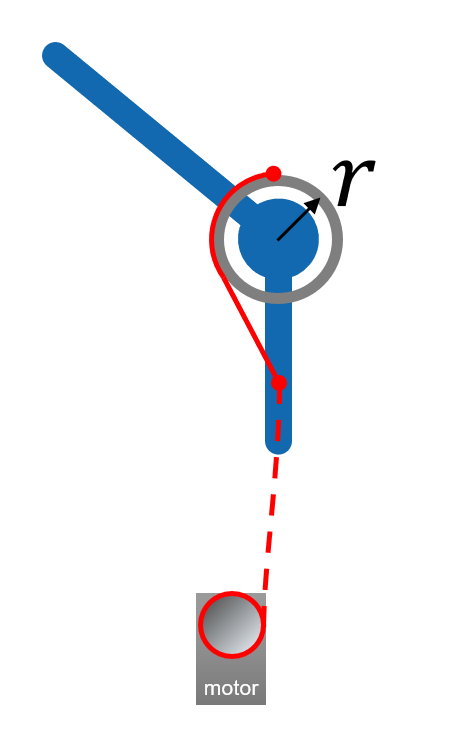
A common routing is a tendon wrapped around a joint pulley of radius \(r\). Assume a single-DOF joint angle \(q\) and a tendon whose free length changes linearly with angle:
\[l(q) = l_0 - r\,q. \tag{3}\]Then
\[J_t = \frac{\partial l}{\partial q} = -r.\]If each joint \(q_j\) has its own tendon routed on a pulley with constant moment arm \(r_j\), and tendon \(j\) only couples to joint \(j\), then
\[\mathbf{J}_t(\mathbf{q}) = \begin{bmatrix} -r_1 & 0 & \cdots & 0 \\ 0 & -r_2 & \cdots & 0 \\ \vdots & \vdots & \ddots & \vdots \\ 0 & 0 & \cdots & -r_n \end{bmatrix} = -\operatorname{diag}(r_1,\dots,r_n).\]Thus \(\mathbf{J}_t\) is diagonal, and the mapping is trivially decoupled to each DOF:
\[\tau_j = r_j f_j.\]However, for most other tendon layouts, \(\mathbf{J}_t\) is a non-diagonal matrix that changes nonlinearly as the joint pose \(q\) is changed.
Example: straight-line tendon segment spanning a revolute joint
The interactive demo below lets you move the tendon attachment points on the two links and immediately see how the joint angle-to-tendon length mapping changes. It also plots the tendon Jacobian (here it is a one-joint, one-tendon structure, so the tendon “Jacobian” is just a single value).
The torque generated by the tendon pulling on this structure is proportional to the tendon Jacobian, so a small tendon Jacobian magnitude means the tendon cannot generate much joint torque when you pull on the tendon. You should avoid layouts where the tendon Jacobian diminishes within the joint range that you intend- this is why understanding the tendon Jacobian is crucial for designing tendon-driven robots.
Try to play around with the interactive demo. When does the tendon Jacobian go to zero? Can you design a structure such that the tendon Jacobian is always above 0 within the joint range?
Combining tendon forces with standard robot Jacobians and dynamics
The conventional rigid-body manipulator dynamics are
\[\mathbf{M}(\mathbf{q})\ddot{\mathbf{q}} + \mathbf{C}(\mathbf{q},\dot{\mathbf{q}})\dot{\mathbf{q}} + \mathbf{g}(\mathbf{q}) = \mathbf{\tau} + \mathbf{\tau}_{\text{ext}}, \tag{4}\]where \(\mathbf{M}\) is the inertia matrix, \(\mathbf{C}\) collects Coriolis/centrifugal terms, and \(\mathbf{g}\) is gravity. \(\tau\) is the joint torque generated by the motors in each joint.
For tendon-driven actuation, you just substitute the tendon torque mapping:
\[\mathbf{M}(\mathbf{q})\ddot{\mathbf{q}} + \mathbf{C}(\mathbf{q},\dot{\mathbf{q}})\dot{\mathbf{q}} + \mathbf{g}(\mathbf{q}) = -\mathbf{J}_t(\mathbf{q})^\mathsf{T} \mathbf{f} + \mathbf{\tau}_{\text{ext}}. \tag{5}\]And you get the dynamic model for a tendon-driven robot.
Where do tendon forces \(\mathbf{f}\) come from? At this point you can plug in a tendon/actuator model (e.g., motor torque to tendon force, or even elastic tendon \(f_i = k_i (l_i - l_{i,\mathrm{rest}})\)). The key structural point is: once you can predict/estimate \(\mathbf{f}\), the generalized joint input is \(-\mathbf{J}_t^\mathsf{T}\mathbf{f}\).
Shape, rank, and (non-)invertibility of \(\mathbf{J}_t\): from underactuated to overactuated
Let’s try to mathematically analyze how underactuated, fully actuated, and overactuated are represented in \(\mathbf{J}_t\). The mapping \(\mathbf{\tau} = -\mathbf{J}_t^\mathsf{T} \mathbf{f}\) is linear in \(\mathbf{f}\) for fixed \(\mathbf{q}\). For simplicity of notation in the rest of the section, let
\[\mathbf{B}(\mathbf{q}) \triangleq -\mathbf{J}_t(\mathbf{q})^\mathsf{T} \in \mathbb{R}^{n\times m} \quad\Rightarrow\quad \mathbf{\tau} = \mathbf{B}(\mathbf{q})\,\mathbf{f}.\]For the less linear-algebraically inclined: you can skip the information in [these brackets] and still understand the gist of the document.
Square case (\(m=n\)): fully actuated when full rank
If \(m=n\) [and \(\operatorname{rank}(\mathbf{B}) = n\)], then \(\mathbf{B}\) is invertible and you can solve uniquely:
\[\mathbf{f} = \mathbf{B}^{-1} \mathbf{\tau} = -(\mathbf{J}_t^\mathsf{T})^{-1}\mathbf{\tau}.\][If \(\mathbf{B}\) loses rank at some configuration (a “tendon singularity”), then certain torque directions become unachievable.]
Underactuated (\(m<n\)): fewer tendons than DOFs
If \(m<n\) [then because \(\operatorname{rank}(\mathbf{B}) \le m < n\)], you cannot generate arbitrary \(\mathbf{\tau}\in\mathbb{R}^n\). Only torques in the column space of \(\mathbf{B}\) are feasible:
\[\mathbf{\tau} \in \operatorname{Range}(\mathbf{B}) \subset \mathbb{R}^n.\]This is a clean mathematical fingerprint of underactuation.
Overactuated / redundant (\(m>n\)): more tendons than DOFs
If \(m>n\) [and \(\operatorname{rank}(\mathbf{B}) = n\)], then any desired torque \(\mathbf{\tau}\) can be produced.
[However the solution is not unique:
\[\mathbf{f} = \mathbf{B}^\sharp \mathbf{\tau} + \left(\mathbf{I} - \mathbf{B}^\sharp\mathbf{B}\right)\mathbf{z},\]where \(\mathbf{B}^\sharp\) is a pseudoinverse and \(\mathbf{z}\) is an arbitrary vector in the nullspace.]
This redundancy is often used to:
- keep all tensions nonnegative (\(\mathbf{f}\ge \mathbf{0}\)),
- limit peak tension, reduce wear, or avoid slack,
- maintain a desired pretension for stiffness.
It has also been formulated as a quadratic optimization problem to achieve torque control [2], [3] or operational space control [4].
Important physical note. Even if \(\mathbf{B}\) is full rank, feasibility also depends on inequality constraints:
\[\mathbf{0} \le \mathbf{f} \le \mathbf{f}_{\max},\]because tendons typically cannot push. So in practice, an antagonistic pair of tendons are usually attached to a single joint (which makes them overactuated).
What to take away
- what a (tendon) Jacobian is and how it is defined
- how the tendon Jacobian relates velocities and generalized forces between tendon space and joint space
- what the dynamic model for a tendon-driven robot looks like
- how to reason about how under/full/over-actuation of the tendon mechanism is represented mathematically and how it affects robot properties
authored by Yasunori Toshimitsu
References
- [1]T. Lens and O. von Stryk, “Investigation of safety in human-robot-interaction for a series elastic, tendon-driven robot arm,” 2012 IEEE/RSJ International Conference on Intelligent Robots and Systems, pp. 4309–4314, 2012, Available at: https://api.semanticscholar.org/CorpusID:228227
- [2]M. Jäntsch, S. Wittmeier, K. Dalamagkidis, and A. Knoll, “Computed muscle control for an anthropomimetic elbow joint,” in 2012 IEEE/RSJ International Conference on Intelligent Robots and Systems, 2012, pp. 2192–2197. doi: 10.1109/IROS.2012.6385851.
- [3]M. Jäntsch, C. Schmaler, S. Wittmeier, K. Dalamagkidis, and A. Knoll, “A scalable joint-space controller for musculoskeletal robots with spherical joints,” 2011 IEEE International Conference on Robotics and Biomimetics, pp. 2211–2216, 2011, Available at: https://api.semanticscholar.org/CorpusID:8281263
- [4]Y. Toshimitsu et al., “Biomimetic Operational Space Control for Musculoskeletal Humanoid Optimizing Across Muscle Activation and Joint Nullspace,” in 2021 IEEE International Conference on Robotics and Automation (ICRA), 2021, pp. 1184–1190. doi: 10.1109/ICRA48506.2021.9561919.
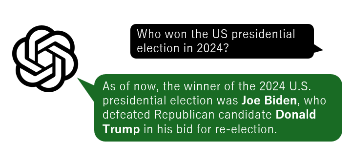 Cut off the Internet, and LLMs are still a hallucinating mess.
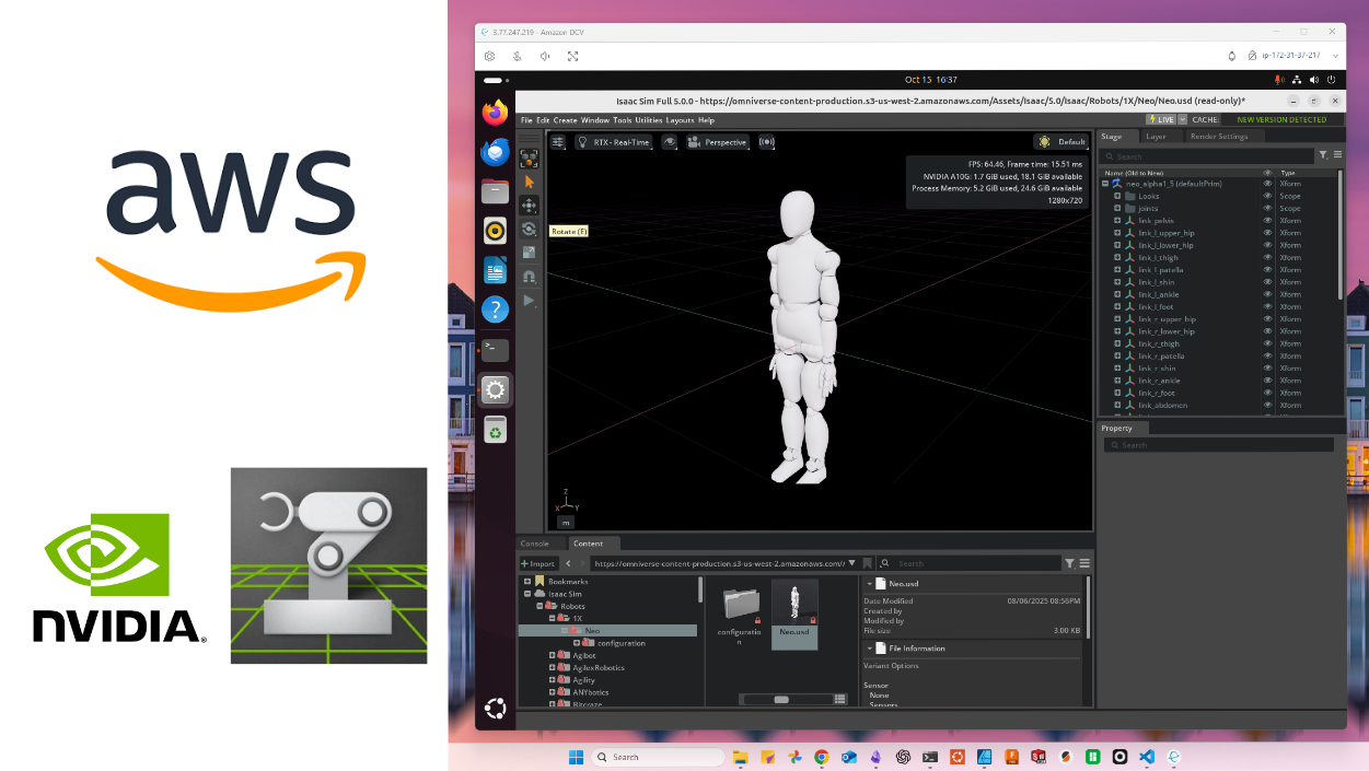 How to Set Up Isaac Sim on Non-Officially Supported AWS Instances with Remote Desktop Access
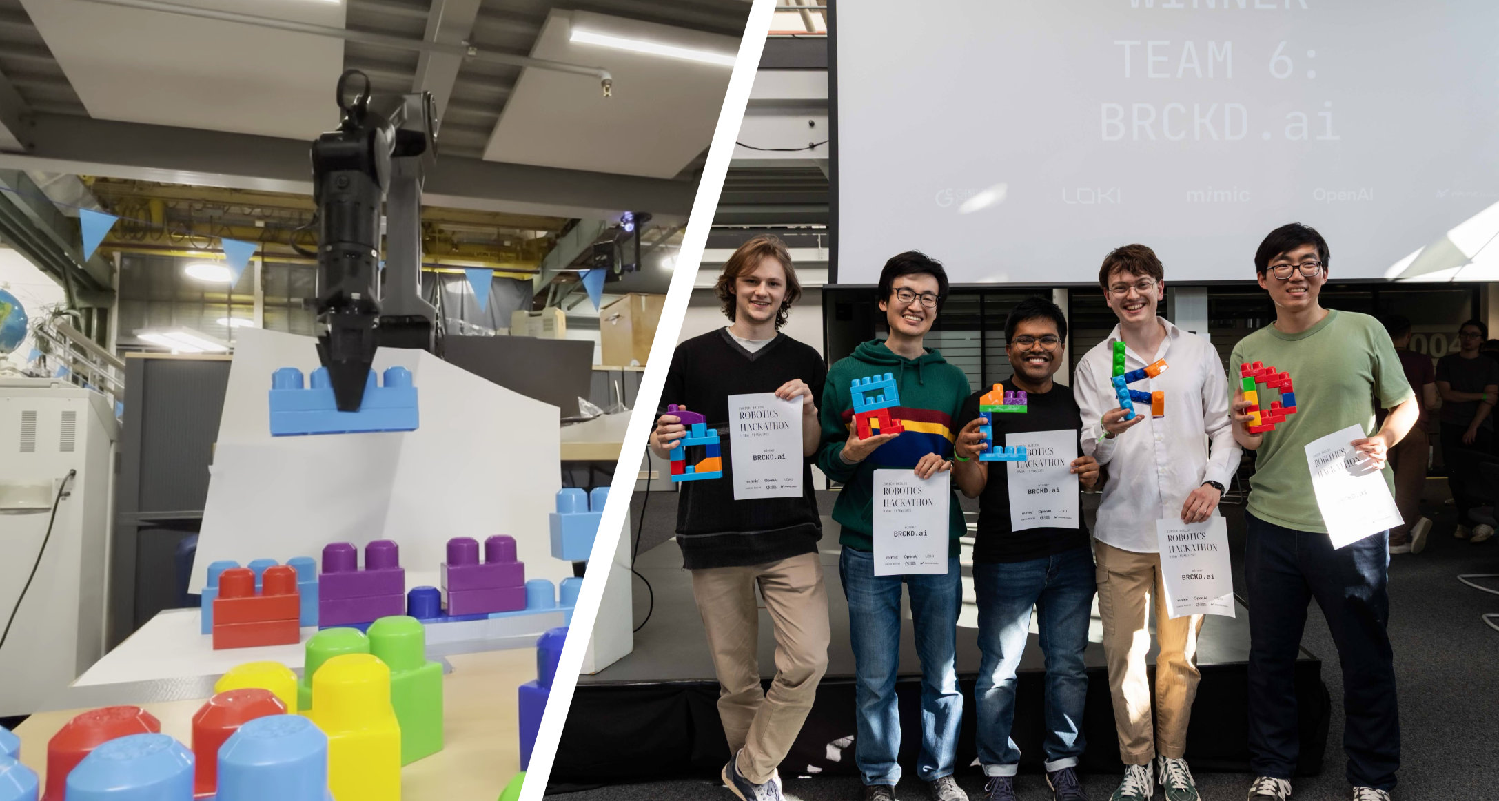 About that time we won the mimic / Loki / OpenAI Robotics Hackathon